Reading from a single file¶

PyGeode was intended for dealing with large gridded datasets - nearly always such datasets will be serialized on disk, sometimes in a single file, but often spread over many files. PyGeode supports a number of different formats, and the commands for loading and saving data to disk are to a large extent independent of the format used, and attempts are made to automatically detect which format you are working with. This being said, NetCDF files are the most completely supported. We’ll start by looking at reading a single file.

In [1]: import pygeode as pyg, numpy as np

In [2]: ds = pyg.open('sample_data/file.nc')

In [3]: print(ds)
<Dataset>:
Vars:
  Temp (lat,lon)  (31,60)
Axes:
  lat <Lat>      :  90 S to 90 N (31 values)
  lon <Lon>      :  0 E to 354 E (60 values)
Global Attributes:
{}

$ ncdump -h file.nc
netcdf file {
dimensions:
  lat = 31 ;
  lon = 60 ;
variables:
  double lat(lat) ;
    lat:units = "degrees_north" ;
    lat:standard_name = "latitude" ;
    lat:ancillary_variables = "lat_weights" ;
    lat:axis = "Y" ;
  double lon(lon) ;
    lon:units = "degrees_east" ;
    lon:standard_name = "longitude" ;
    lon:axis = "X" ;
  double Temp(lat, lon) ;
  double lat_weights(lat) ;

// global attributes:
    :history = "Synthetic Temperature data generated by pygeode" ;
}

In [4]: print(ds.lat.weights)
[6.12323400e-17 1.04528463e-01 2.07911691e-01 3.09016994e-01
 4.06736643e-01 5.00000000e-01 5.87785252e-01 6.69130606e-01
 7.43144825e-01 8.09016994e-01 8.66025404e-01 9.13545458e-01
 9.51056516e-01 9.78147601e-01 9.94521895e-01 1.00000000e+00
 9.94521895e-01 9.78147601e-01 9.51056516e-01 9.13545458e-01
 8.66025404e-01 8.09016994e-01 7.43144825e-01 6.69130606e-01
 5.87785252e-01 5.00000000e-01 4.06736643e-01 3.09016994e-01
 2.07911691e-01 1.04528463e-01 6.12323400e-17]

Overriding metadata¶

All of this is convenient when one has a well-formed NetCDF file, however, one often encounters rather bare NetCDF files in the wild, with either no or (even worse) incorrect metadata. In this case PyGeode will not be able to recognize what kind of Axis it should associate with each each axis:

In [5]: from pygeode.tutorial import t1

In [6]: pyg.save('sample_data/file_nometa.nc', t1, cfmeta=False)

In [7]: ds2 = pyg.open('sample_data/file_nometa.nc')

In [8]: print(ds2)
<Dataset>:
Vars:
  Temp (lat,lon)  (31,60)
Axes:
  lat <NamedAxis 'lat'>:  -90  to 90  (31 values)
  lon <NamedAxis 'lon'>:  0  to 354  (60 values)
Global Attributes:
{}


In [9]: pyg.showvar(ds2.Temp)
Out[9]: <pygeode.plot.wrappers.AxesWrapper at 0x7f37340173a0>

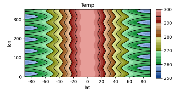
The lat and lon axes are now the default type NamedAxes. While this is still a perfectly useable PyGeode dataset, PyGeode no longer knows how to properly annotate and format plots.

However, if you know what the contents of the file represent, you can provide this information to PyGeode when opening it by passing special keyword arguments to open(). The most important of this is the dimtypes argument, which takes a dictionary whose keys are the names of the axes in the file being opened, and whose values tell PyGeode what kind of Axis class to associate with that dimension. This is perhaps best illustrated by example:

In [10]: dt = dict(lat = pyg.Lat, lon = pyg.regularlon(60))

In [11]: print(pyg.open('sample_data/file_nometa.nc', dimtypes=dt))
<Dataset>:
Vars:
  Temp (lat,lon)  (31,60)
Axes:
  lat <Lat>      :  90 S to 90 N (31 values)
  lon <Lon>      :  0 E to 354 E (60 values)
Global Attributes:
{}

We can see that now the NamedAxis objects have been replaced by the appropriate axis types, Lat and Lon, respectively. You will notice we have used two different ways of specifying the axes types. In the case of lat, we have simply passed the PyGeode class itself. In this case, PyGeode reads the values for the lat dimension from the file and uses these to create a new instance of Lat.

In contrast, for the lon axis, we have created an instance of the Lon class (with a helper function regularlon()) prior to opening the file. In this case, PyGeode simply uses the already-created axis, and avoids reading in the coordinates for the axis being overridden. Of course, the length of the axis must mach the length of the dimension in the file. This is useful for when the data in the file is not correct, but it can also happen that in very large files, depending on the details of how the file data has been structured, even just reading the coordinate metadata can be quite a slow operation. If you regularly work with such a file, passing in an already created axis instance can speed up call to open the file considerably.

There is one more form that can be used in the dimtypes dictionary, for when one wants to construct an axis using data from the file, but when the axis type in question requires additional arguments to be properly constructed. To give a contrived example, consider the following code (which is unfortunately a bit opaque):

In [12]: kwargs = dict(units='days', startdate = dict(year=2001, month=1, day=1))

In [13]: dt2 = dict(lon = (pyg.StandardTime, kwargs))

In [14]: print(pyg.open('sample_data/file_nometa.nc', dimtypes=dt2))
<Dataset>:
Vars:
  Temp (lat,time)  (31,60)
Axes:
  lat <NamedAxis 'lat'>:  -90  to 90  (31 values)
  time <StandardTime>:  Jan 1, 2001 00:00:00 to Dec 21, 2001 00:00:00 (60 values)
Global Attributes:
{}

Here we have decided to treat the lon axis describing a time axis, but for some reason we wish to use the coordinate data as actual time information. As will be explained in more detail in a later section (Working with Axes), time axes generally need a bit more information when they are constructed to define the calendar. We need give these additional arguments (the units and startdate items in the kwargs dictionary) which we pass in along with the class object itself. PyGeode then calls the constructor of the StandardTime with the values read from the file and with the additional keyword arguments to create a new axis object, which is then assigned to the lon dimension of any variable.

There are a few other arguments recognized by open(), but we’ll just mention one more, perhaps the second most useful: namemap. This allows you to simply rename variables and axes:

In [15]: nm = dict(lon = 'Longitude', Temp='Temperature')

In [16]: print(pyg.open('sample_data/file_nometa.nc', namemap=nm, dimtypes=dt))
<Dataset>:
Vars:
  Temperature (lat,Longitude)  (31,60)
Axes:
  lat <Lat>      :  90 S to 90 N (31 values)
  Longitude <Lon>:  0 E to 354 E (60 values)
Global Attributes:
{}

As you can see, the original axes names as defined in the file are still used to replace axis types in the dimtypes dictionary; the axis is renamed after it has been replaced by the newly specified axis class.

Reading from multiple files¶

PyGeode is intended for use with very large datasets, which are often distributed across many files. It has two additional methods, openall() and open_multi(), which are intended for use with such datasets. The first, which is the simpler of the two, is better suited for moderately large datasets which consist of multiple files, but not a large number of files. This works by opening each file explicitly, then merging the contents of each file into a single PyGeode dataset. Since each file is explicitly opened and its metadata read in, this can add up for datasets consisting of a large number of files. A subtler issue is that the concatenation PyGeode uses in this case is also, at present, somewhat less efficient than it could be. As a result, accessing the data opened with this method is not as fast as the second method.

The second, open_multi(), is somewhat more complicated to use, but is better suited for very large datasets, particularly in which the dataset is separated along the time axis. In this case PyGeode simply opens the first and last file in the dataset, reads in their metadata, then infers the contents of the rest of the files given an addition (user-defined) function that maps filenames to dates. Since only two files are opened, this is a very efficient operation even for extremely large datasets. As was just mentioned, the data is also loaded more efficiently than from datasets opened with the first method.

To demonstrate these two methods, we’ll need a sample dataset to work with. To keep the dataset small, we’ll write out the zonal mean of the temperature field from the second tutorial dataset, one year per file

In [17]: from pygeode.tutorial import t2

In [18]: for y in range(2011, 2021):
   ....:   pyg.save('sample_data/temp_zm_y%d.nc' % y, t2.Temp(year=y).mean('lon'))
   ....: 

This produces ten files, each with a year of data in them.

To demonstrate openall(), we can simply provide a wildcard filename which matches the filenames:

In [19]: ds = pyg.openall('sample_data/temp_zm_*.nc', namemap=dict(Temp='T'))

In [20]: print(ds.T)
<Var 'T'>:
  Shape:  (time,pres,lat)  (3650,20,31)
  Axes:
    time <ModelTime365>:  Jan 1, 2011 00:00:00 to Dec 31, 2020 00:00:00 (3650 values)
    pres <Pres>    :  1000 hPa to 50 hPa (20 values)
    lat <Lat>      :  90 S to 90 N (31 values)
  Attributes:
    {}
  Type:  SortedVar (dtype="float64")

PyGeode expands the wildcard, opens each of the files, then concatenates the datasets. The result is a single dataset object with 10 years of temperature data that you can use without worrying further about how the data is distributed on disk. The filenames can alternatively be specified as a list; in fact in this case PyGeode expands each item in the list if there are wildcards (using glob.glob()).

The same arguments (dimtypes and namemap) apply; here we’ve renamed the variable Temp to T. In addition, if you need to do more sophisticated manipulations of the data in each file before PyGeode concatenates the individual datasets, you can provide a function that takes the filename (as a string) as a single argument, and returns the modified dataset. This can be useful, for instance, for correcting issues in individual files:

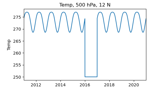
In [21]: def opener(f):
   ....:   ds = pyg.open(f)
   ....:   if '2016' in f: # Replace the data in this file with a dummy value
   ....:     return pyg.Dataset([ds.Temp * 0 + 250.])
   ....:   else:
   ....:     return ds
   ....: 

In [22]: ds = pyg.openall('sample_data/temp_zm_*.nc', opener=opener)

In [23]: pyg.showvar(ds.Temp(lat=15, pres=500))
Out[23]: <pygeode.plot.wrappers.AxesWrapper at 0x7f373411aca0>

Using open_multi() is in most respects very similar. The main difference is that in addition to specifying the filenames, this method assumes that the dataset is divided along the time axis, and you need to provide a way for PyGeode to map each filename to a date.

In simple cases this can be done by simply specifying a regular expression that matches the components of the date in the filename. For instance:

In [24]: patt = 'temp_zm_y(?P<year>[0-9]{4}).nc'

In [25]: print(pyg.open_multi('sample_data/temp_zm_*.nc', pattern=patt))
<Dataset>:
Vars:
  Temp (time,pres,lat)  (3650,20,31)
Axes:
  time <ModelTime365>:  Jan 1, 2011 00:00:00 to Dec 31, 2020 00:00:00 (3650 values)
  pres <Pres>    :  1000 hPa to 50 hPa (20 values)
  lat <Lat>      :  90 S to 90 N (31 values)
Global Attributes:
{}

The regular expression matches the four digit year in the filenames in a way that PyGeode can understand. Since this four digit format is commonly encountered, there is an abbreviation for it you can use which saves you the trouble of remembering how Python regular expressions work:

In [26]: patt = 'temp_zm_y$Y.nc'

In [27]: print(pyg.open_multi('sample_data/temp_zm_*.nc', pattern=patt))
<Dataset>:
Vars:
  Temp (time,pres,lat)  (3650,20,31)
Axes:
  time <ModelTime365>:  Jan 1, 2011 00:00:00 to Dec 31, 2020 00:00:00 (3650 values)
  pres <Pres>    :  1000 hPa to 50 hPa (20 values)
  lat <Lat>      :  90 S to 90 N (31 values)
Global Attributes:
{}

Similar abbreviations exist for 2-digit month, day, hour, and minute fields (see open_multi() for details), though if the filenames you’re working with aren’t in the appropriate format, you’ll have to provide the full regular expression.

In some cases the filenames themselves don’t quite have enough information, or else it’s difficult to write an appropriate regular expression to parse out the right information. As an alternative, you can also specify a Python function that takes the filename as an argument, and returns the corresponding date dictionary. As a simple example,

In [28]: def f2d(fn):
   ....:   date = dict(month=1, day=1)
   ....:   date['year'] = int(fn[-7:-3]) # Extract the year from the filename and convert to an integer
   ....:   return date
   ....: 

In [29]: print(pyg.open_multi('sample_data/temp_zm_*.nc', file2date = f2d))
<Dataset>:
Vars:
  Temp (time,pres,lat)  (3650,20,31)
Axes:
  time <ModelTime365>:  Jan 1, 2011 00:00:00 to Dec 31, 2020 00:00:00 (3650 values)
  pres <Pres>    :  1000 hPa to 50 hPa (20 values)
  lat <Lat>      :  90 S to 90 N (31 values)
Global Attributes:
{}

Note that in the interests of speed, PyGeode only opens the first and last file in the dataset, and then infers the contents of the remainder of the files. The assumption is made that the contents of each file are identical, only translated in time. If there are errors or missing data in the interior files, these will not be detected when opening the dataset. It is good practice when opening such a dataset for the first time to explicitly load in at least some of the data from each file in the dataset to confirm that all the files are well-formed. There is a helper function for this purpose, pygeode.formats.multifile.check_multi().

Saving to files¶

In contrast to reading files, saving PyGeode variables and datasets to disk is typically a much simpler operation, and we’ve seen examples of this already in a couple places in this tutorial. The save() method takes a filename and either a single Var object, or a Dataset object (in fact it uses the helper function asdataset() which recognizes various other kinds of collections of variables as well). As with reading files, writing to NetCDF files is the best supported option. By default, PyGeode writes NetCDF version 3 format files for greater compatibility, but this version has a number of limitations, including a maximum file size. Alternatively, version 4 format files can be written by specifying

In [30]: pyg.save('sample_data/file_v4.nc', t1, version=4)

which permits larger files to be written. There are several other options, including built-in compression (this is a feature of the NetCDF 4 library), and packing, which can be done in any format. See save() for details.

If you have a large dataset you wish to write out in multiple files, you can simply select the subset you wish before saving the variable or dataset to disk.