Getting Started¶

We’ll start by taking a look at a couple of synthetic datasets defined in the tutorial module of PyGeode. The first such dataset can be imported as follows:

In [1]: import pygeode as pyg

In [2]: from pygeode.tutorial import t1

In [3]: print(t1)
<Dataset>:
Vars:
  Temp (lat,lon)  (31,60)
Axes:
  lat <Lat>      :  90 S to 90 N (31 values)
  lon <Lon>      :  0 E to 354 E (60 values)
Global Attributes:
  history        : Synthetic Temperature data generated by pygeode

The dataset t1 contains one pygeode variable object, Temp, which is defined on a two dimensional grid of 31 latitudes and 60 longitudes. The grid is defined by the two pygeode axes objects, lat and lon, which span from 85 S to 85 N, and from 0 E to 354 E. respectively.

We can take a closer look at our variable Temp:

In [4]: print(t1.Temp)
<Var 'Temp'>:
  Units: K  Shape:  (lat,lon)  (31,60)
  Axes:
    lat <Lat>      :  90 S to 90 N (31 values)
    lon <Lon>      :  0 E to 354 E (60 values)
  Attributes:
    {}
  Type:  Add_Var (dtype="float64")

Again, we see both physical and numerical details of the grid on which this variable is defined, as well that the temperatures are defined in degrees Kelvin.

Finally, we can look as well at one of our axes:

In [5]: print(t1.lat)
lat <Lat>      :  90 S to 90 N (31 values)

which we could also access as a member of the variable Temp: t1.Temp.lat.

These three types of objects, variables, axes, and datasets, are the core of PyGeode. Variables (Var) encapsulate a scalar field such as temperature or one component of the wind field. Axes (Axis), which are in fact special cases of variables, define the geophysical grid on which the scalar field exists. Finally, datasets (Dataset) are containers for variables. These concepts match reasonably closely to their counterparts in NetCDF files (and indeed PyGeode works very naturally with NetCDF files). We’ll learn more about all three soon, but to get a quick feel of what PyGeode can do, let’s try plotting the contents of our first variable:

# Depending on what python interpreter you are using, you may need to run
# these commands to access the plotting functionality of matplotlib
In [6]: import pylab as pyl; pyl.ion();

In [7]: pyg.showvar(t1.Temp)
Out[7]: <pygeode.plot.wrappers.AxesWrapper at 0x7f37362c5070>

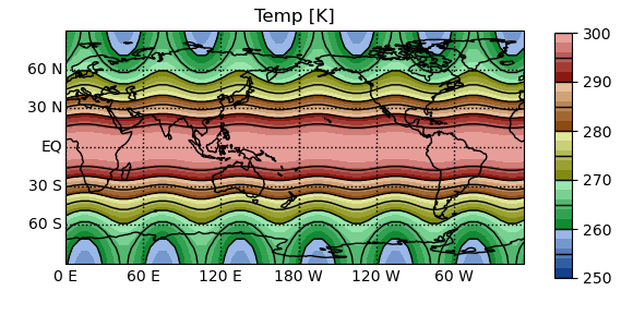
PyGeode annotates the axes automatically, and if the Cartopy package is installed, data on a lat-lon grid is plotted over the outline of the continents using a cylindrical projection. All plots generated by PyGeode are in fact generated using the matplotlib library; the plotvar command simply makes many educated guesses about the type of plot you might want to generate based on the variable you’ve passed in. Many aspects of the plot can be customized through the plotvar interface (which we’ll get into later on in this tutorial), but if you find you can’t tweak things just so, the plot can always be manipulated using the matplotlib library itself which gives you full control.

Now let’s take a look at a second dataset:

In [8]: from pygeode.tutorial import t2

In [9]: print(t2)
<Dataset>:
Vars:
  Temp (time,pres,lat,lon)  (3650,20,31,60)
  U    (time,pres,lat,lon)  (3650,20,31,60)
Axes:
  time <ModelTime365>:  Jan 1, 2011 00:00:00 to Dec 31, 2020 00:00:00 (3650 values)
  pres <Pres>    :  1000 hPa to 50 hPa (20 values)
  lat <Lat>      :  90 S to 90 N (31 values)
  lon <Lon>      :  0 E to 354 E (60 values)
Global Attributes:
  history        : Synthetic Temperature and Wind data generated by pygeode

This is a somewhat more complicated temperature field, now defined on four dimensions: time, pressure, latitude and longitude. Note this grid has over 350 million data points–enough that the 2010-era laptop this tutorial was first written on would complain if we attempted to load all of it into memory at once. This brings us to one of the major guiding assumptions of pygeode - that since we haven’t done anything that needs the data itself, none of it has yet been loaded or computed. We can, nonetheless, manipulate this variable as if it has:

In [10]: Tc = pyg.climatology(t2.Temp)    # Compute the climatology

In [11]: Tcz = Tc.mean('lon')        # Compute the zonal mean

In [12]: print(Tcz)
<Var 'Temp_clim_mean'>:
  Shape:  (time,pres,lat)  (365,20,31)
  Axes:
    time <ModelTime365>:  Jan 1,  00:00:00 to Dec 31,  00:00:00 (365 values)
    pres <Pres>    :  1000 hPa to 50 hPa (20 values)
    lat <Lat>      :  90 S to 90 N (31 values)
  Attributes:
    {}
  Type:  MeanVar (dtype="float64")

In [13]: Tcp = Tc - Tcz              # Compute anomaly from the zonal mean

In [14]: Tcp = Tcp.rename("T'")      # Rename variable

In [15]: print(Tcp)
<Var 'T''>:
  Shape:  (time,pres,lat,lon)  (365,20,31,60)
  Axes:
    time <ModelTime365>:  Jan 1,  00:00:00 to Dec 31,  00:00:00 (365 values)
    pres <Pres>    :  1000 hPa to 50 hPa (20 values)
    lat <Lat>      :  90 S to 90 N (31 values)
    lon <Lon>      :  0 E to 354 E (60 values)
  Attributes:
    {}
  Type:  RenamedVar (dtype="float64")

We’ve now computed (at least an abstract sense) the climatolgical anomaly from the zonal mean. Note that Tcz is defined on a reduced grid (we’ve lost the Lon axis), and it looks and behaves just like any other PyGeode variable; PyGeode has some automatic logic for properly aligning Tc and Tcz when taking their difference. However, no data has yet been loaded, no actual averages have been taken, and no differences computed, since we haven’t done anything that needs the data. If we now go and plot the near-surface, high-latitude anomaly of our synthetic dataset:

In [16]: pyg.showvar(Tcp(pres=1000, time='15 Jun 00'))
Out[16]: <pygeode.plot.wrappers.AxesWrapper at 0x7f37341da700>

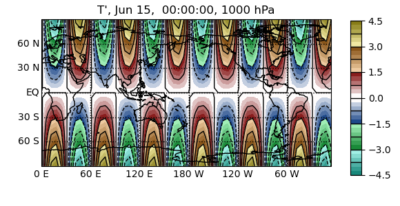
We now actually need to perform these operations (though only on one pressure level and one latitude), so PyGeode goes back and accesses the required data (only), then carries out all of our operations before sending the data off to matplotlib to produce a nice contour plot.

Implied in the operations above is another principle of PyGeode. Note that nowhere did we need to remember which dimension of an array corresponded to time and which corresponded to longitude; nor did we need to know what index described the 1000 hPa pressure level, or which corresponded to the 15th of June. Moreover, we could take the difference between two fields (Tc and Tcz) which weren’t defined on the same grid–PyGeode takes care of the broadcasting and alignment of the underlying numpy arrays for us, leaving us to think about the problem we’re trying to solve in the physical coordinate space of our data. The underlying mapping is of course still there, and if it’s ever more convenient to think in the space of the data arrays, you are still free to do so; the relevant syntax and commands are described later in this tutorial.

‘This is all fine and good,’ you may be thinking, ‘but how do I work with my own data?’ PyGeode supports a number of data formats, though it works most naturally with NetCDF (or HDF5) files. As an example, the synthetic dataset used above can be written out to a NetCDF file (this assumes that a subdirectory called ‘sample_data’ already exists in your working directory):

In [17]: pyg.save('sample_data/file.nc', t1)

and then read back in using:

In [18]: ds = pyg.open('sample_data/file.nc')

In [19]: print(ds)
<Dataset>:
Vars:
  Temp (lat,lon)  (31,60)
Axes:
  lat <Lat>      :  90 S to 90 N (31 values)
  lon <Lon>      :  0 E to 354 E (60 values)
Global Attributes:
{}

PyGeode is aware of the metadata in the file and constructs variables and axes accordingly, following the CF metadata standard used for climate data. Datasets that span multiple files can be handled as well, and one can tailor these calls so that PyGeode properly recognizes your data regardless of the metadata in the file.

This concludes the introductory tutorial. We’ve seen the three basic objects in PyGeode: variables (Var), axes (Axis) and datasets (Dataset). We’ve seen examples of how PyGeode carries out all operations in a ‘lazy’ fashion, delaying all loading and processing of data until the output is explicitly required. We’ve seen a few examples of the automatic annotation of plots that PyGeode takes care of for you, and finally we’ve seen how to save and load data to a file. The next part of these tutorials gives a deeper introduction to the Basic Operations that one can perform on PyGeode variables.