Selecting subsets¶

Reference: Var.__call__()

One of the most basic operations is to select a subset or subdomain of your variable. For instance, to select a rectangular region of the same temperature variable we just saw:

In [6]: print(t1.Temp(lat=(30, 50), lon=(100, 180)))
<Var 'Temp'>:
  Units: K  Shape:  (lat,lon)  (4,14)
  Axes:
    lat <Lat>      :  30 N to 48 N (4 values)
    lon <Lon>      :  102 E to 180 E (14 values)
  Attributes:
    {}
  Type:  SlicedVar (dtype="float64")

# We can take a look at the latitude grid points for reference
In [7]: t1.Temp.lat[:]
Out[7]: 
array([-90., -84., -78., -72., -66., -60., -54., -48., -42., -36., -30.,
       -24., -18., -12.,  -6.,   0.,   6.,  12.,  18.,  24.,  30.,  36.,
        42.,  48.,  54.,  60.,  66.,  72.,  78.,  84.,  90.])

PyGeode makes use of the calling syntax of Python to do slicing. While this is arguably an abuse of the syntax, this operation is so common that it’s a default behaviour for PyGeode variables. The axes are specified as keyword arguments, and ranges are given as a tuple in coordinate space (as opposed to the indices). Not all axes need be specified: any axes not mentioned are left alone. Note that the subset includes elements lying on and within the boundaries of the range requested (30 N to 50 N in this case). To demonstrate this we’ve printed out the grid points of the latitude axis in line 6; so one can see that this call returns a subset from latitude 30 N (on the boundary of the range requested) to 48 N, since the next grid point is at 54 N.

You can also request a single element. The returned variable will always have the same number of dimensions as the source variable (in the same order, though not necessarily the same length), even if some of them are of length 1.

In [8]: print(t1.Temp(lat=12))
<Var 'Temp'>:
  Units: K  Shape:  (lat,lon)  (1,60)
  Axes:
    lat <Lat>      :  12 N
    lon <Lon>      :  0 E to 354 E (60 values)
  Attributes:
    {}
  Type:  SlicedVar (dtype="float64")

If the (zero-based) index is more convenient, you can specify this by prefixing the axis name with i_:

In [9]: print(t1.Temp(i_lat=5).lat)
lat <Lat>      :  60 S

Negative values index the axes in reverse, as in Python:

In [10]: print(t1.Temp(i_lat=-5).lat)
lat <Lat>      :  66 N

Another useful prefix is l_, which lets you select an arbitrary set of points:

In [11]: print(t1.Temp(l_lat=(-25, 0, 60, 92)).lat.values)
[-24.   0.  60.  90.]

You’ll notice that if the requested value lies between two grid points in the subsetted axis (lat in this case), the closer of the two will be returned. This is also the case for values lying outside the range of the axis - this can lead to some surprises if the axes has a different range than you expect. This ‘nearest match’ behaviour only holds for floating-point valued axes - integer-valued axes (such as those that might index members of an ensemble, for instance) only return exact matches.

The subsetted axis will always retain the order of the source axis, regardless of what order you give the list. There are some other useful shortcuts here, but we’ll introduce them a bit later on. In most cases, these prefix shortcuts can be combined, so that li_ can be used to select a list based on indices of the subsetted axes instead of values.

Time axes are a bit of special case. PyGeode has a reasonably sophisticated time axis, which is aware of four types of calendars - the standard Gregorian calendar (StandardTime), a 365-day calendar (ModelTime365), a 360-day calendar (ModelTime360), and a yearless calendar (Yearless), which might better be described as a time axis with no calendar at all. The example data set t2, for instance, is defined on a 365-day calendar. These are represented internally as a list of offsets (in this case in days) from a reference date:

In [12]: from pygeode.tutorial import t2

In [13]: print(t2.time.startdate)
{'year': 2011, 'month': 1, 'day': 1, 'hour': 0, 'minute': 0, 'second': 0}

In [14]: print(t2.time.values)
[0.000e+00 1.000e+00 2.000e+00 ... 3.647e+03 3.648e+03 3.649e+03]

Time axes can be subsetted exactly as above, in which case the requested value is matched against this offset:

In [15]: print(t2.Temp(time=8).time)
time <ModelTime365>:  Jan 9, 2011 00:00:00

However, these can be difficult to use directly, and can easily correspond to very different dates if two time axes have different reference dates. Other possibilities exist:

# Select a range of dates, from 12 December 2013 to 18 January 2014
In [16]: print(t2.Temp(time=('12 Dec 2013', '18 Jan 2014')).time)
time <ModelTime365>:  Dec 12, 2013 00:00:00 to Jan 18, 2014 00:00:00 (38 values)

PyGeode also recognizes the format 16:00 13 May 1982 if a more precise specification is required.

# Select all elements in year 2013
In [17]: print(t2.Temp(year = 2013).time)
time <ModelTime365>:  Jan 1, 2013 00:00:00 to Dec 31, 2013 00:00:00 (365 values)

# Select all elements in any January, February or December
In [18]: print(t2.Temp(l_month = (1, 2, 12)).time)
time <ModelTime365>:  Jan 1, 2011 00:00:00 to Dec 31, 2020 00:00:00 (900 values)

These last two are particularly useful constructs; you will have noticed that axes need not be regularly spaced. Note that year and month here are not axes of t2.Temp – they are technically ‘auxilliary arrays’ of the time axis; this detail doesn’t much matter for users, except that while in most cases they behave exactly as if they were an axis for the purpose of subsetting variables, not all prefixes work. In particular the prefix i_ is not recognized. day, hour, minute, and second work in the same way. More details about time axes can be found here Time Axis Operations.

These examples all return a new PyGeode variable, as explained at the beginning of the section. If you ever do just need the raw numerical data (in the form of a numpy array), you can use standard slicing notation on a pygeode variable (t1.Temp[:] will return everything). Note that, unlike keyword-based subsetting, but like the behaviour expected with selecting out of numpy arrays, degenerate axes are removed in this unlike numpy slicing, degenerate axes are removed. That is, t1.Temp[0, 1] returns a scalar, while t1.Temp(i_lat=0, i_lon=1) returns a two dimensional variable.

Arithmetic operations and broadcasting rules¶

Reference: Element-wise math and Arithmetic Operations on Variables

Arithmetic and other mathematical operations are also supported by PyGeode. The simplest are unary operations, which are performed elementwise. Most standard mathematical functions (powers, exponentials, trigonometric functions, etc.) are supported, and can be found in the main pygeode module:

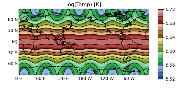
In [19]: pyg.showvar(pyg.log(t1.Temp))     # Plot the natural logarithm of Temp
Out[19]: <pygeode.plot.wrappers.AxesWrapper at 0x7f3735e40430>

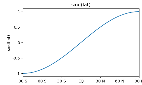
There are some convenience functions included, for instance, most trig functions have a version which takes arguments in degrees rather than radians:

In [20]: pyg.showvar(pyg.sind(t1.lat))     # Compute the sine of latitude
Out[20]: <pygeode.plot.wrappers.AxesWrapper at 0x7f3734399550>

In most cases the underlying operation is performed by the numpy equivalent, though there are a few additional operations as well. A full list can be found in Element-wise math. The PyGeode wrappers are designed to properly handle PyGeode variables, so one should get accustomed to including the pyg prefix. This is also a good reason to import pygeode into its own namespace, rather than into the top-level namespace itself.

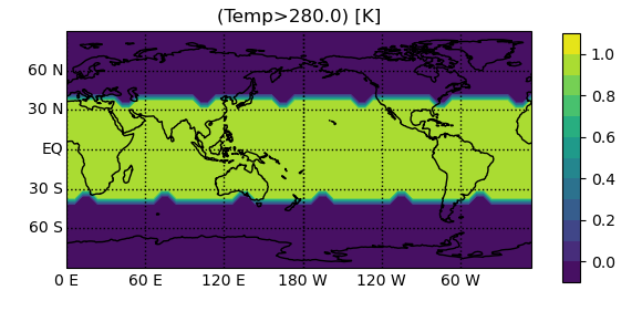
Standard Python binary arithmetic operations (+, -, *, /, **, etc.) are supported and work as one would expect if all the variables are defined on the same axes. Comparison operators (>, <, etc.) are also supported and produce a boolean variable on the same axes with the result of the operation performed elementwise. This can be very useful for masking data, since when cast to scalar values, True is equal to 1 and False is equal to 0:

In [21]: import numpy as np

In [22]: pyg.showvar(t1.Temp > 280., clevs=np.arange(-0.1, 1.11, 0.1))
Out[22]: <pygeode.plot.wrappers.AxesWrapper at 0x7f3734322430>

If the variables do not share the same axes, PyGeode follows a set of rules for automatically broadcasting them so that the operations behave as one might typically desire - it’s important to be aware of these rules as you can sometimes end up with some unexpected results, so they are described here in some detail.

In [23]: print((t2.U + t2.Temp).axes)   # No broadcasting required
(<ModelTime365>, <Pres>, <Lat>, <Lon>)

In [24]: print((t2.lat + t2.lon).axes)  # Broadcast to (lat, lon)
(<Lat>, <Lon>)

In [25]: print((t2.lon + t2.lat).axes)  # Broadcast to (lon, lat)
(<Lon>, <Lat>)

In [26]: print((t2.lon + t2.Temp).axes)  # Broadcast to (time, pres, lat, lon)
(<ModelTime365>, <Pres>, <Lat>, <Lon>)

# Broadcasting restricts longitude axis to subset
In [27]: print((t2.Temp(lon=(0, 180)) - t2.Temp).lon)
lon <Lon>      :  0 E to 180 E (31 values)

# Subsetted longitude axes are not compatible:
In [28]: try: print((t2.Temp(lon=(0, 180)) + t2.Temp(lon=(120, 240))).lon)
   ....: except ValueError as e: print(e)
   ....: 
Axes <lon <Lon>      :  120 E to 240 E (21 values)> and <lon <Lon>      :  0 E to 180 E (31 values)> cannot be mapped.

Reductions (Averages, Standard deviations)¶

As we saw at the beginning of this section, you can compute averages over a variable with mean(). By default this computes an average over the whole domain, but you can specify particular axes you want to average over. For example,

In [29]: print(t2.Temp.mean('pres', pyg.Lon))
<Var 'Temp'>:
  Shape:  (time,lat)  (3650,31)
  Axes:
    time <ModelTime365>:  Jan 1, 2011 00:00:00 to Dec 31, 2020 00:00:00 (3650 values)
    lat <Lat>      :  90 S to 90 N (31 values)
  Attributes:
    {}
  Type:  MeanVar (dtype="float64")

This computes an average over the both the pressure and longitude axes. You can specify axes in three ways:

• by name, e.g. t2.Temp.mean('lon')

• by class, e.g. t2.Temp.mean(pyg.Lon)

• or by (zero-based) index, e.g. t2.Temp.mean(3)

These will all (in this case) return the same average. These three ways of identifying axes are pretty general across PyGeode routines.

Often it’s useful to compute an average over a subset of the domain. You could first select the subdomain, then compute the mean (t2.Temp(lat=(70, 90)).mean('lat')), but this is such a common operation that there is a short cut in the form of another selection prefix, m_:

In [30]: print(t2.Temp(m_lat=(70, 90)))
<Var 'Temp'>:
  Shape:  (time,pres,lon)  (3650,20,60)
  Axes:
    time <ModelTime365>:  Jan 1, 2011 00:00:00 to Dec 31, 2020 00:00:00 (3650 values)
    pres <Pres>    :  1000 hPa to 50 hPa (20 values)
    lon <Lon>      :  0 E to 354 E (60 values)
  Attributes:
    {}
  Type:  WeightedMeanVar (dtype="float64")

This selects all latitudes between 70 N and 90 N and performs an average.

You may notice this last operation returned a WeightedMeanVar, rather than just a MeanVar. PyGeode, by default, will perform weighted averages over axes which have weights associated with them. In this case, our latitude axis is weighted its cosine, to take in to account the smaller surface area near the poles:

In [31]: print(t2.Temp.lat.weights)
[6.12323400e-17 1.04528463e-01 2.07911691e-01 3.09016994e-01
 4.06736643e-01 5.00000000e-01 5.87785252e-01 6.69130606e-01
 7.43144825e-01 8.09016994e-01 8.66025404e-01 9.13545458e-01
 9.51056516e-01 9.78147601e-01 9.94521895e-01 1.00000000e+00
 9.94521895e-01 9.78147601e-01 9.51056516e-01 9.13545458e-01
 8.66025404e-01 8.09016994e-01 7.43144825e-01 6.69130606e-01
 5.87785252e-01 5.00000000e-01 4.06736643e-01 3.09016994e-01
 2.07911691e-01 1.04528463e-01 6.12323400e-17]

You can turn this off, if desired, by specifying weights=False as a keyword argument:

In [32]: print(t2.Temp.mean('lat', weights=False))
<Var 'Temp'>:
  Shape:  (time,pres,lon)  (3650,20,60)
  Axes:
    time <ModelTime365>:  Jan 1, 2011 00:00:00 to Dec 31, 2020 00:00:00 (3650 values)
    pres <Pres>    :  1000 hPa to 50 hPa (20 values)
    lon <Lon>      :  0 E to 354 E (60 values)
  Attributes:
    {}
  Type:  MeanVar (dtype="float64")

Alternatively, you can specify your own weights to use, in the form of a PyGeode variable with the same axes as those you would like to weight:

In [33]: print(t2.Temp.mean('lat', weights=pyg.sind(t2.Temp.lat)))
<Var 'Temp'>:
  Shape:  (time,pres,lon)  (3650,20,60)
  Axes:
    time <ModelTime365>:  Jan 1, 2011 00:00:00 to Dec 31, 2020 00:00:00 (3650 values)
    pres <Pres>    :  1000 hPa to 50 hPa (20 values)
    lon <Lon>      :  0 E to 354 E (60 values)
  Attributes:
    {}
  Type:  WeightedMeanVar (dtype="float64")

The weights do not need to be normalized; PyGeode will do that automatically.

There are several other axes reductions that behave similarly, including Var.stdev(), Var.variance(), Var.sum(), Var.min(), Var.max(); see Axis Reductions for the full list. Some differences exist though:

• Var.sum() by default does not use the axes weights; you can use the default weights by specifying weights=True as a keyword argument.

• Var.max() and Var.min() do not use weights; they return the maximum and minimum values (respectively) along the axes being reduced.

Finally, there are also equivalents for several of these methods which are NaN aware.

Reshaping variables¶

Finally, there are a whole set of basic manipulations you can perform on variables if you need to rework their structure. Some of the most common are introduced here; for a complete list see Array manipulation routines. Keep in mind that variables are thought of as immutable objects - that is, once they’re created, they don’t change - as before, what the following operations actually do is return a new variable with the desired changes that wraps the old one.

Var.transpose() reorders the axes of a variable. Not all axes need to be specified; those that are not will be appended in their present order.

In [34]: t2.Temp.axes
Out[34]: (<ModelTime365>, <Pres>, <Lat>, <Lon>)

In [35]: print(t2.Temp.transpose('lon', 'lat', 'pres', 'time').axes)
(<Lon>, <Lat>, <Pres>, <ModelTime365>)

Var.replace_axes() replaces any or all axes of a variable. The new axes must have the same length as those they are replacing.

# The logPAxis method returns a log-pressure axis with a given scale height
In [36]: print(t2.Temp.replace_axes(pres=t2.pres.logPAxis(H=7000)).axes)
(<ModelTime365>, <ZAxis>, <Lat>, <Lon>)

Var.squeeze() removes degenerate axes (those with one or fewer elements). As mentioned above, the default selection behaviour is to always return a variable with the same number of axes as you’ve started with, even if those axes have only a single element. If you want to remove these degenerate axes, you can use this command, which, when called with no arguments, will simply remove all degenerate axes. Several other methods of calling are also available:

# Squeeze all degenerate axes
In [37]: print(t2.Temp(time = 4, lon = 20).squeeze())
<Var 'Temp'>:
  Shape:  (pres,lat)  (20,31)
  Axes:
    pres <Pres>    :  1000 hPa to 50 hPa (20 values)
    lat <Lat>      :  90 S to 90 N (31 values)
  Attributes:
    {}
  Type:  SqueezedVar (dtype="float64")

# Squeeze only the time axis (if it is degenerate)
In [38]: print(t2.Temp(time = 4, lon = 20).squeeze('time'))
<Var 'Temp'>:
  Shape:  (pres,lat,lon)  (20,31,1)
  Axes:
    pres <Pres>    :  1000 hPa to 50 hPa (20 values)
    lat <Lat>      :  90 S to 90 N (31 values)
    lon <Lon>      :  18 E
  Attributes:
    {}
  Type:  SqueezedVar (dtype="float64")

# Select a single value then squeeze the time axis
In [39]: print(t2.Temp.squeeze(time = 4))
<Var 'Temp'>:
  Shape:  (pres,lat,lon)  (20,31,60)
  Axes:
    pres <Pres>    :  1000 hPa to 50 hPa (20 values)
    lat <Lat>      :  90 S to 90 N (31 values)
    lon <Lon>      :  0 E to 354 E (60 values)
  Attributes:
    {}
  Type:  SqueezedVar (dtype="float64")

# Select a single value and sqeeze the time axis using a selection prefix
In [40]: print(t2.Temp(s_time = 4, lon = (20, 40)))
<Var 'Temp'>:
  Shape:  (pres,lat,lon)  (20,31,3)
  Axes:
    pres <Pres>    :  1000 hPa to 50 hPa (20 values)
    lat <Lat>      :  90 S to 90 N (31 values)
    lon <Lon>      :  24 E to 36 E (3 values)
  Attributes:
    {}
  Type:  SqueezedVar (dtype="float64")

There are also commands to rename variables and their axes (Var.rename(), Var.rename_axes()), for adding axes to a variable (Var.extend()), reordering axes elements (Var.sorted()) and dealing with NaNs (Var.fill(), Var.unfill()).